Single-Agent Search: How Does AI Solve a Maze

Introduction

In single-agent search problems, the goal is usually for an AI to come up with a sequence of actions that leads to the solution. In other words, in order to let an AI solve a puzzle, for instance, a maze, the program has to perform a search for a path (or paths) that leads itself from the starting point all the way down to the goal. The question is: How? And how do various aproaches differ from one another?

Overview

Before we start, here is a simple interpretation of how the computer is solving a maze.

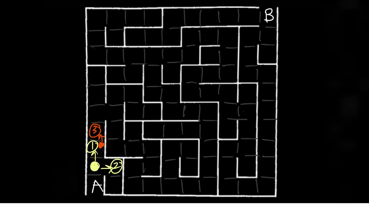
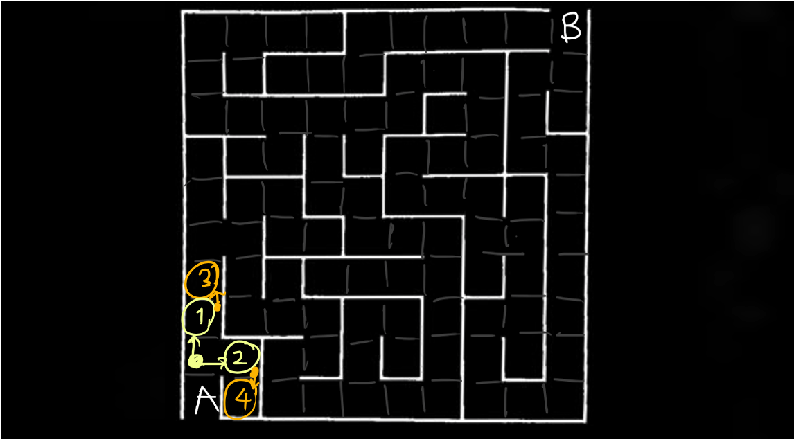
• Suppose you start at point A and want to go to point B. There is not much choice for the first step because the computer can only move one step upward (to the yellow dot).
• Then, you can either ① go up or ② go right.
• Suppose you choose ①, and you realized it is still not the goal. You then keep searching.

Now you are at orange dot which your list of choice becomes ② and ③. It means that you can either continue with your journey to the north, or you can go back to the last choice to choose ②. That is because you haven’t explored ② yet. Maybe it’s the goal to the maze so it’s totally reasonable go back and check.

But which way to go next? ② or ③? That's where searching algorithms kick in.

There exists a full range of ways to perform a search. In this reading, some fundamental searching algorithms will be introduced:

• Depth-First Search
• Breadth-First Search
• Greedy Best-First Search
• A* Search

They all have unique propertities which will be dicussed in the next part.

---

Types of Search

1. Depth-First Search (DFS)

In Depth-First Search, you must stick along with the latest decision you made until you reach a dead end. In other words, you do not go back until you exhaust the whole path. Therefore, ③ is the right place to go, instead of ②.

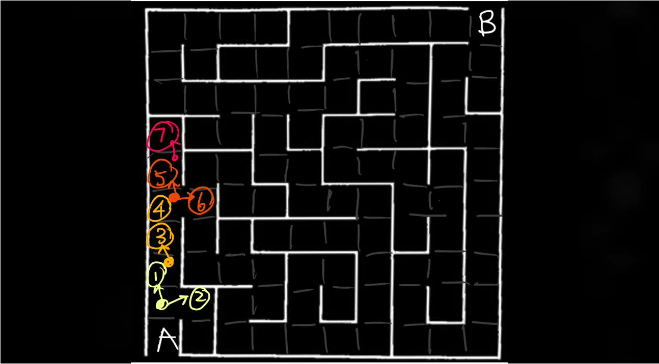
Similarly, at ③, you can either go to ④ or go back to choose to go to ②. Sticking along with the latest decision, ④ would be the reasonable place to go under Depth-First Search.

At ④, you now have choices of checking ②, ⑤, and ⑥.

According to the logic that has brought us to come to ④, we should consider ⑤ or ⑥. Suppose we pick to go to ⑤ and we have ②, ⑥, and ⑦ to choose. We choose ⑦, finally coming to a dead end.

At this point we have exhausted the whole path, leaving ② and ⑥ the current choices. Now we take one step backward and continue sticking with the latest possible choice ⑥.

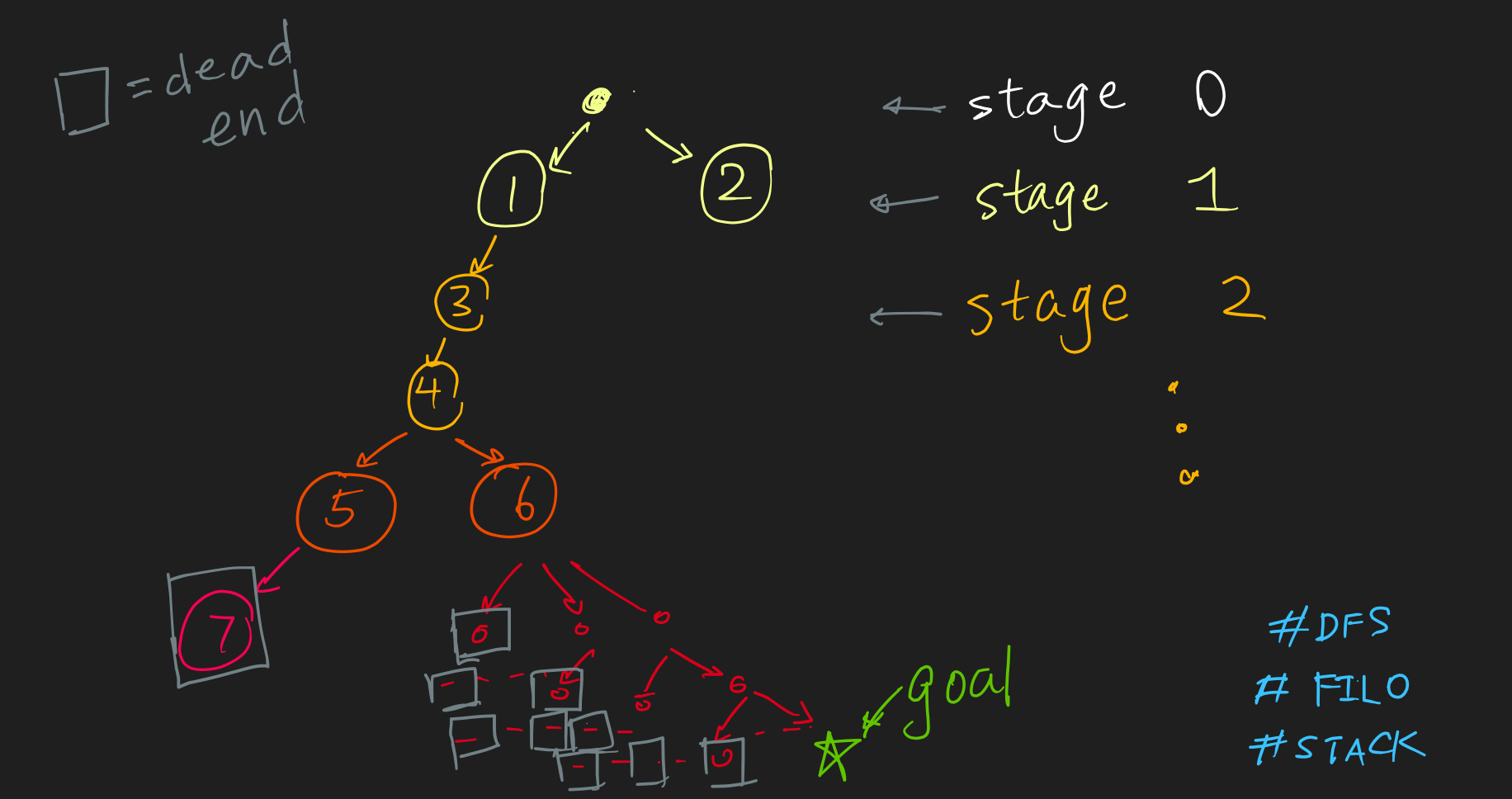
If we look at the moves stage by stage, you can see that the computer will eventually find the goal after meeting all the dead ends it can possibly meet. Also, you will notice that the computer would never actually choose to go to ② because it would have already found the goal before that even happens.

2. Breadth-First Search (BFS)

The second search algorithm we are looking at is Breadth-First Search (BFS). It is very much like Depth-First Search. The only difference is, instead of stacking the choices and picking the latest one, Breadth-First Search lets the choices queue and always picks the oldest one.

Let’s take a look at how exactly BFS works. We still start from the yellow dot and can pick between going to ① or ② at time zero. Suppose we still go with ① for now.

Then, we can choose between going to ③, or ②. Since ② is older in the queue, we pick ② this time.

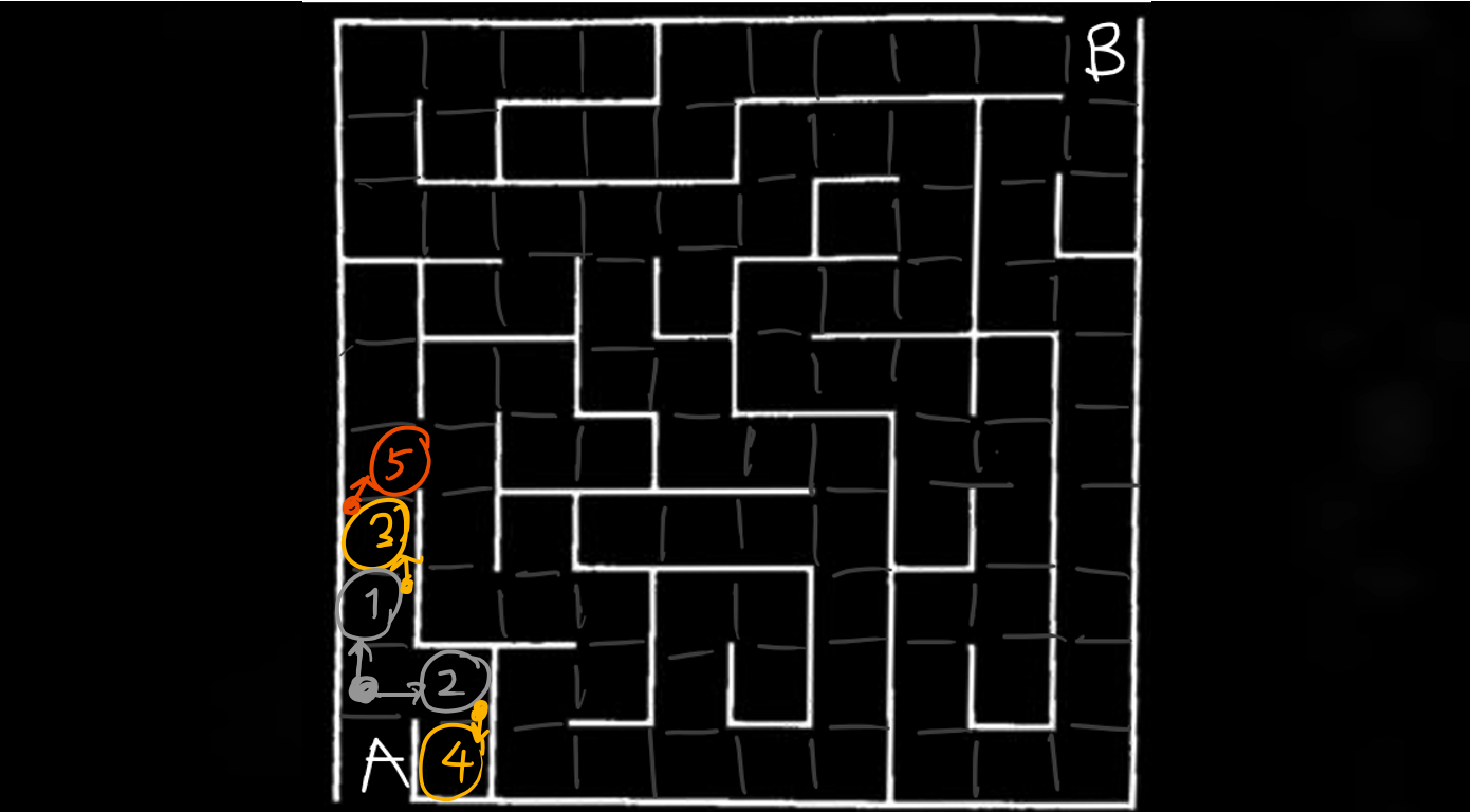
And now, we can either go to ③ or ④. Since ③ is older in our queue, we go to ③, adding ⑤ into our queue. Then we explore ④. ④ is checked and is found to be a dead end. We go to our only choice - ⑤ , adding ⑥ and ⑦ to the list.

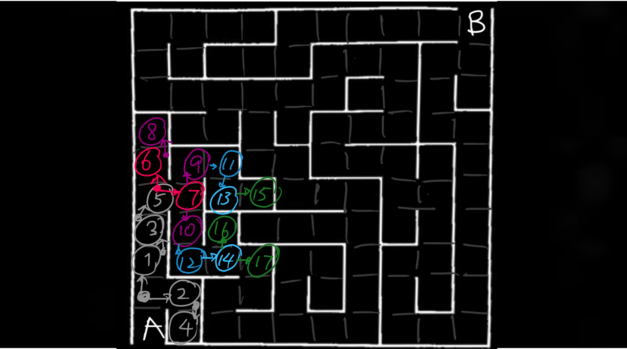
Go to ⑥, add ⑧, then go to ⑦, and add ⑨⑩.

Then ⑪⑫ , ⑬⑭, and ⑮⑯⑰ in alternating path, and so on, until you reach the goal.

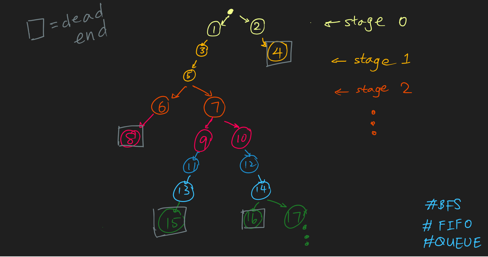
Tree representation of Breadth-Depth Search:

In fact, the computer can be smarter. It can use the given information as a “hint” for where to go next. In a problem like maze, the position of the goal can serve well as “given information”. That’s where the third type of search comes in – Greedy Best-First Search.

3. Greedy Best-First Search

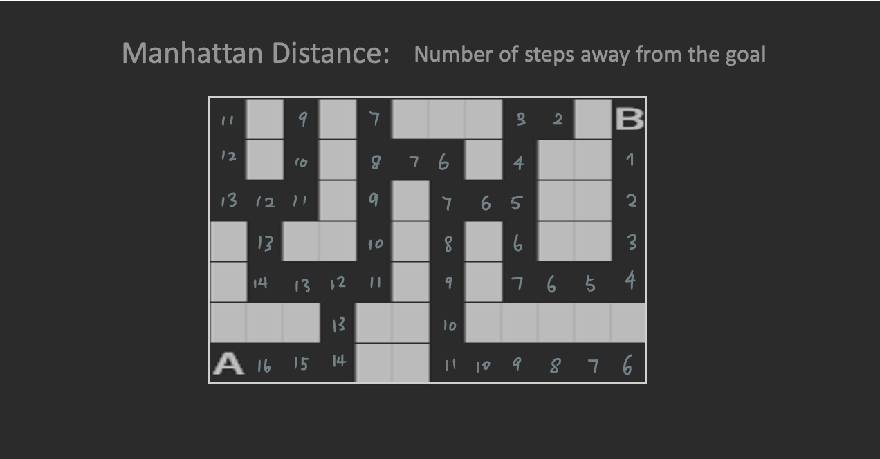
In Greedy Best-First Search, a value of the Manhattan distance is assigned to each cell. It tells you how far the cell is away from the goal and hence, gives you an “inkling” of where you should go next.

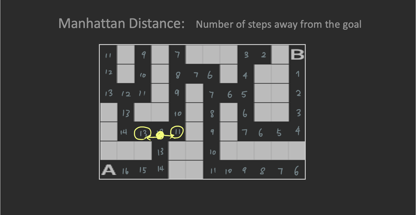
Whenever the computer has to choose among the choice list of where to go next, this algorithm always pick the one with the shortest Manhattan distance. That’s why it is called Greedy Best-First.

For instance, I am at ⑫ now and have to choose between going left and going right. This algorithm would take me to the right because it has a shorter Manhattan distance ⑪ than ⑬.

4. A* Search

Finally, the last search to be introduced is A* search. You can think of it as an “upgraded” version of Greedy Best-First Search, because not only does it take Manhattan Distance into account, but it also keeps track of the cost – number of steps that have taken you from the starting point to your current location.

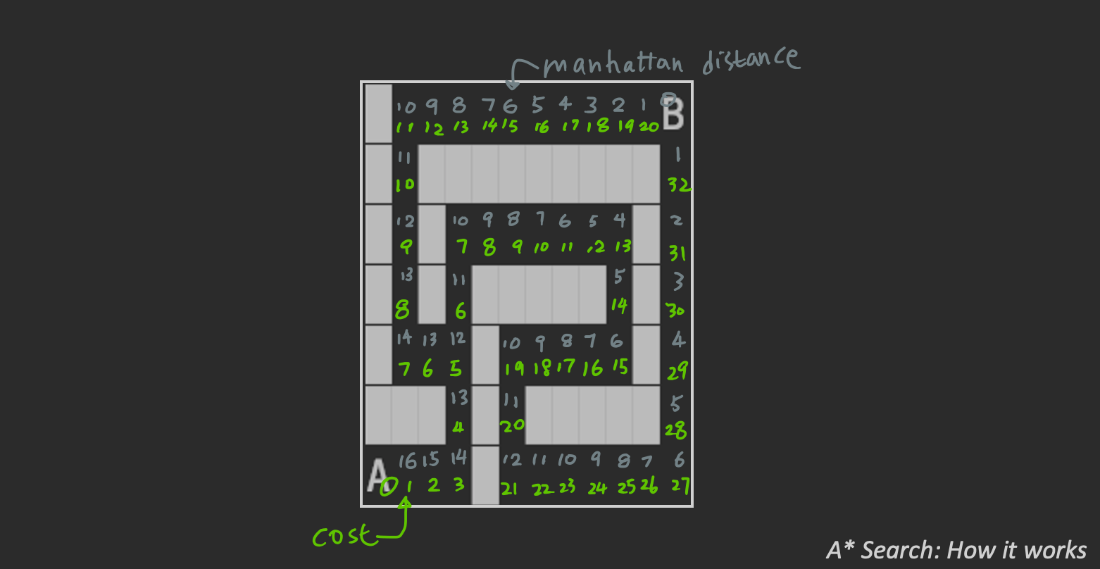
Logically you want to find a shorter path, which is another saying of “to minimize your cost”. In the picture, the green value is the cost function of every cell. The longer it is away from the starting point A, the larger the cost. For the longer path it costs 32 steps go to from point A to B, but it only costs 20 steps for the shorter path.

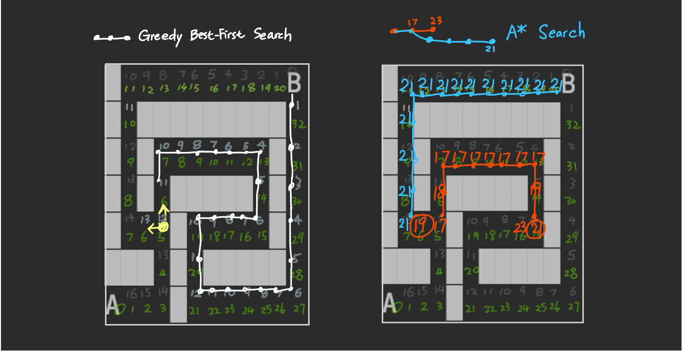
Suppose you came across to the first crossroad at yellow dot. Greedy Best-First Search would have guided you upward, all the way down to point B, letting you finish the longer path. That is because if we look at the Manhattan values in gray along the longer path, not a single cell has a greater gray value than 13, the Manhattan value of your choice of going left from the yellow dot.

But in A* Search, we combine the Manhattan distance and the cost function. The combined value in the middle of the long path (21) exceeded the value of 19, circled in red. It means that we've gone a long way, but the goal is not getting closer. In this case we might just abandon the red path, go back to the last crossroad, go for the blue path and finally come to the goal with a shorter path.

---

Why finding which algorithm to use matters?

After all the tedious explanation, it is obvious that different types of algorithm works in different ways. The real problem is: Which one is better? Is queuing always better than stacking? Which one should we choose?

The short answer is: “It depends”. Let's take a look at some examples.

Example - Map

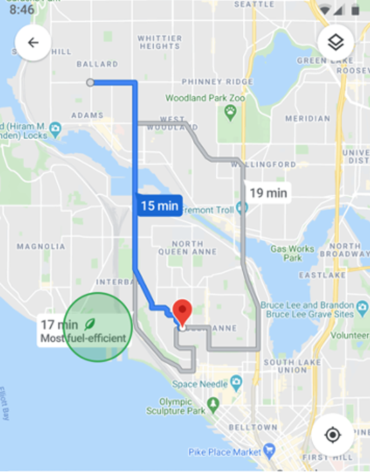
Imagine you are using google map. There are numerous ways that can get you from point A to point B. Neglecting traffic and other road situations, normally you would want to search for the shortest route to the destination. Then which algorithm to pick should depend on which path gives you the shortest distance to get to the destination, so that you can arrive as soon as possible.

Example - Maze

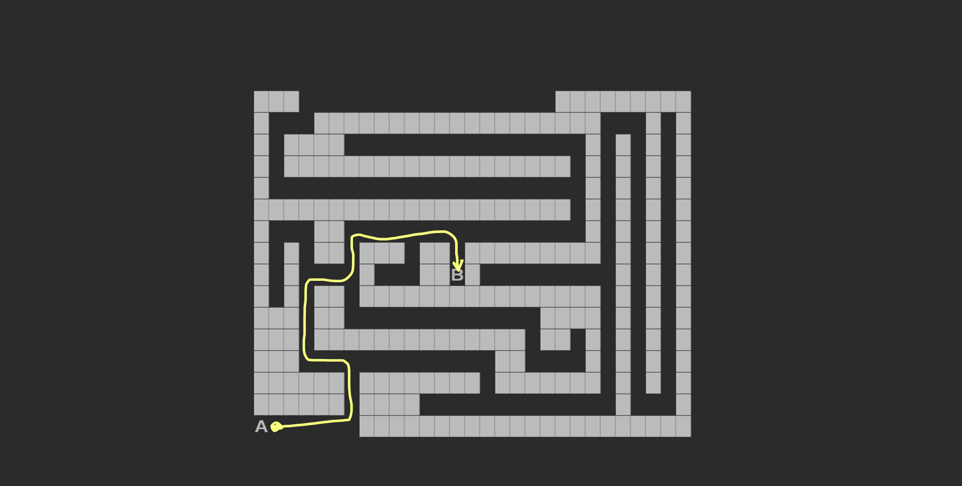
If you are playing a maze game, there is usually only one correct path to your destination. Then maybe you would choose an algorithm that is the least time-consuming than the others in searching for that one route. In this case, searching time (and memory) matters.

---